Table of Contents
1.0 | Using Web Applications to Georeference
2.0 | Introduction to GIS and Historical Data
3.0 | Georeferencing an Historic Map
0.0 | Overview
In this workshop we will be working with images of historic maps, georectifying them to align with contemporary maps, accessing public historic data, and experimenting with web-publishing outputs to combine historic imagery with historic data.
This tutorial requires personal accounts for the following online applications:
MapWarper
Mapbox
Carto
1.0 | Using Web Applications to Georeference
An important distinction we should make from the beginning is between the historic map as an image and the digital maps we know online.
Scanned historic maps and pixels
Online maps and tilesets
The historic image will need to be georeferenced and then georectified to match the pixels of the scanned image to the geographic data that underlies the online images of maps. We will first explore the relationship between these two image types by using a web application available through the New York Public Library: MapWarper.
1.1 | Get the historic map
The imagery [from the New York Public Library collection] has been uploaded to MapWarper, and is ready for us to rectify.
Please go to the link, log into MapWarper, using your personal account:
Map of Dutchess County, New-York from original surveys / J.C. Sidney C.E.
1.2 | Group georeference
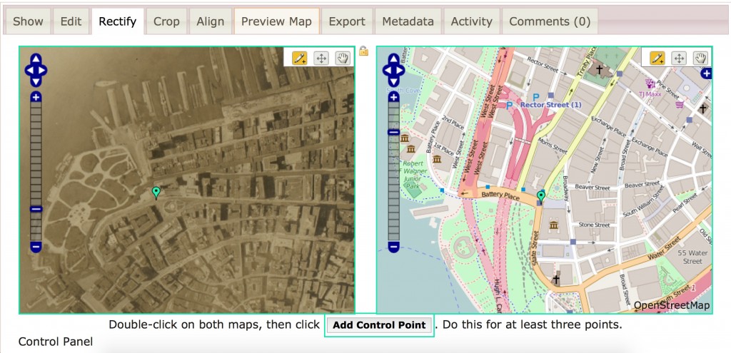
Once you are logged in, click on the tab: Rectify
You will see two panes. The one on the left is the historic imagery; the one on the right is a view of the Open Street Map. To begin georeferencing the historic map, you can click on a point to make a green marker appear, then find the corresponding point on the Open Street Map to make a green marker appear on this map.
To set the points on both maps, click on the button below the two maps: Add Control Point. The points will then be assigned a number.
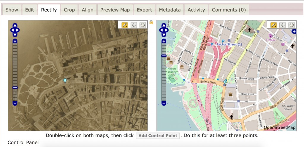
We can do this collectively, but the points added by other collaborators won’t appear automatically. After adding each point, please refresh your browser so that you don’t add points on top of other collaborators’ points.
Be sure to click Add Control Point after locating each point. Then refresh your browser.
1.3 | Using the georeferenced map
Once we have georeferenced several points, one person from the group can then Warp Image. We can use the default settings for image. [Additional settings are available in Advanced Options]
Now we have a georeferenced image that can serve for a number of web-publishing outputs.
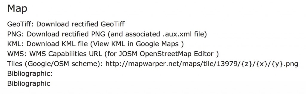
Click on the Export tab to see the various outputs. We can test a few of these outputs.
1.4 | Using Carto for georeferenced map
Log in to Carto to test the map.
First, create a new map by clicking on the blue button to make a New Map.

The next page will be your Datasets page. Click on the blue text: Create empty map

Once you see a map view, we will now add a base layer of the historical map we rectified. Click on the button for the Basemap (by default set to the Positron map).

In the pane on the left, first choose the folded map image for Custom under Source. Then, click on the plus sign under Style to add a new map.

On the next screen, copy and paste this URL into the field (note that the XYZ tab is selected at top)
http://mapwarper.net/maps/tile/15250/{z}/{x}/{y}.png
Select Add Basemap. [Do not click TMS]

You will likely see just a blank gray screen next. Fear not, your map is there. In the search bar at the top right, type in Red Hook, NY (or any town in Dutchess County). You will then seen the map with a red pin marker. You can now zoom in to the image.

1.5 | Using Mapbox for georeferenced image
1.5.a | Tiling your geotiff
This map, unfortunately, has no context of the map’s surroundings. CartoDB does not allow you to add layers of basemaps. However, we can use Mapbox to create a more complex basemap that places the georeferenced image over a contemporary map.
From the MapWarper Export tab, choose to download GeoTiff. Save it to a place you can easily find it again.
Go to Mapbox and log in to your account.
Once at the Dashboard, click on the tab at left for Tilesets. Click the blue button for New tileset.


In the next window that appears, click to Select a file. Navigate to the geotiff you saved from MapWarper and select it.

1.5.b | Styling the basemap
We will have to wait some time for Mapbox to generate tiles from the georeferenced image. As we wait, we can begin to style the context map on which we we place the georeferenced image.
Click on the Styles tab at left. Click on the purple button, New Style. Here you can choose whichever basemap you like. I prefer the Light style, as it is a nice gray background that doesn’t interfere with the imagery of the historic map. Select Create.

We can style some of the features that will work well to overlay the historic image, such as roads and water. First, rearrange these items to the top of the layers list at the left. Bring Roads, Water, Road Labels, and Water Labels to the top. These can each by styled by changing colors, labels, and opacity.
1.5.c | Adding your geotiff to the basemap
By now, the geotiff should have processed and added to your map. Click on + New Layer at the top of the layers panel at left. Click in the field No Tileset to add the georeferenced image. Choose the image from the list.

Once it is added, drag it below the labels you moved to the top area of the layers so that the layers we styled will appear on top of the image.
Now, we can publish the map and view it in CartoDB. Click on the purple Publish button. Choose the teal button, Publish in the next window. Then, Share and Use this Style.
In the next window, we will change the option in the last box to CartoDB. And, then copy the link that appears in the box.

Open CartoDB. Now, choose to change the basemap. In the XYZ option, paste the url just copied from Mapbox. Click Add basemap.
Return to top ↵
2.0 | Introduction to GIS and Historical Data
2.1 | Vectors and Rasters
Geographic Information Systems (GIS) is software that allows you to create geographically accurate (meaning mathematically projected) maps . The beauty of using GIS over other imaging software is that you can create a “thick” map with layers of information that are georeferenced. This software allows you to spatialize the layers of information you may have in a database.
Thus, there are two kinds of data that are stored for each item in GIS:
attribute (the data stored in tables or databases)
spatial (data that is georeferenced / is coordinate based)
Additionally there are two types of spatial data that are distinguished from one another in GIS:
vector (features that are points, lines, or polygons that are attached at coordinates)
raster (continuous surfaces of images in which the pixels are georeferenced)
Now, in QGIS, open the program and click on the blank page icon in the upper left to create a new project.

You will see that the project is blank with no data. Let’s add some data!
2.2 | Retrieving Historical Data
Next, we will be creating a map by adding shape (vector) and TIFF (raster) files from publicly available datasets: CUGIR: Cornell University Geospatial Information Repository and NYS GIS Clearinghouse.
Today we will eventually be working with an historic map of the town of Red Hook, NY, so first we need some data that will contextualize the historic map.
Go to the NYS GIS Clearinghouse for the civil boundaries of New York State. This will give us several shape files (vector files) with data attached to vectors marking the boundaries of counties, cities/towns, villages, etc. Download the SHAPE file by clicking on the link. Save these to a new folder that you create on the desktop.
For the sake of QGIS projects, it is wise to save all the files you use in the project in a single folder. We will be loading several different shape (.shp) files and rasters into a single project as layers. Keeping all these files together in a single place is important because QGIS does not save the files to the project; rather it links to the files. If the link is broken (by moving the files after saving the project) QGIS will have a hard time finding them and will produce errors.

These files all come zipped. Click on them to unzip. Note all the different files that make up a set of data (spatial and attribute): .shx, .shp, .sbx, .sbn, .prj, .dbf, and .cpg These all must stay together so that the attribute data remains attached to the vector data of the shape file.

Now, we need some data for roads, waterways, and railroads. Retrieving this information at the state level would likely be overwhelming. So, we will use CUGIR to get these files at the county level. We will download the hydrography (rivers, ponds, lakes), minor civil boundaries (the townships), the roads, and the railroads zipped files.

These files are zipped and the shape files within are also zipped. Both levels of folders will need to be unzipped to use them.


2.3 | Adding vector layers in QGIS
In QGIS, choose Layer > Add Layer > Add Vector Layer
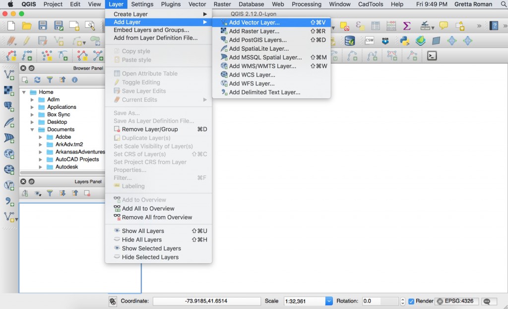
A dialogue box will appear. Keep Source Type as File. Click the button Browse to open a directory. Navigate (where you saved all your shape files) to choose NYS_Civil_Boundaries.shp > Counties_Shoreline.shp. [*Take note of the .shp file extension]
Click Open in this box, and then click Open in the next box, too. The counties and shorelines of New York state will now appear in the right pane of QGIS.

Add the vector layers for the CUGIR data now, too.
You can change the order of the layers in the left panel by dragging the layer to a different spot. I put the minor civil boundaries behind the roads and waterways, for instance.
2.4 | Styling a vector layer
The color of your vector polygons will be random. We can change the color by double-clicking on the layer in the Layer Panel on the bottom left pane. This box will appear with several options for modifying the layer. We will be working under the Style tab (note the other tabs on the left side).
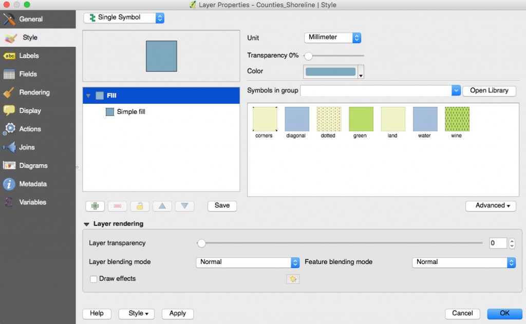
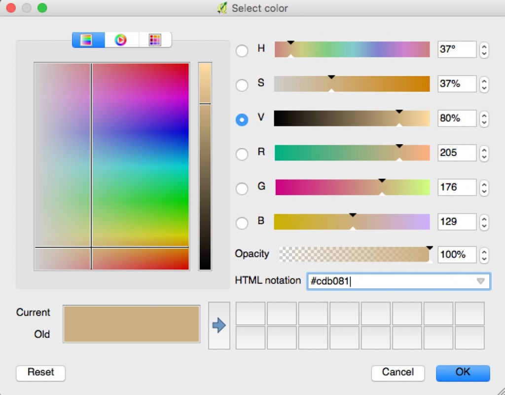
Double-click on bar of color in the field, Color. I have made the vectors of the state’s counties this color: #cdb081. You can change the color by pasting this hex-value in the field, HTML notation. Click OK in the Select color box and then OK in the Layer Properties box.
We can style the layers even more. First, let’s rename the waterways and roads files so we can know the difference more easily. Right click on the layer name, choose Rename, and change it to Waterways_Dutchess and Roads_Dutchess accordingly. (see above for reference)
For Waterways_Dutchess, I changed the color to: #376199. After clicking OK, in the Select Color box, I changed the width of the line to .40 in the Layer Properties box.
For Roads_Dutchess, I changed the color to: #333333. After clicking OK, in the Select Color box, I changed the width of the line to .25 in the Layer Properties box.
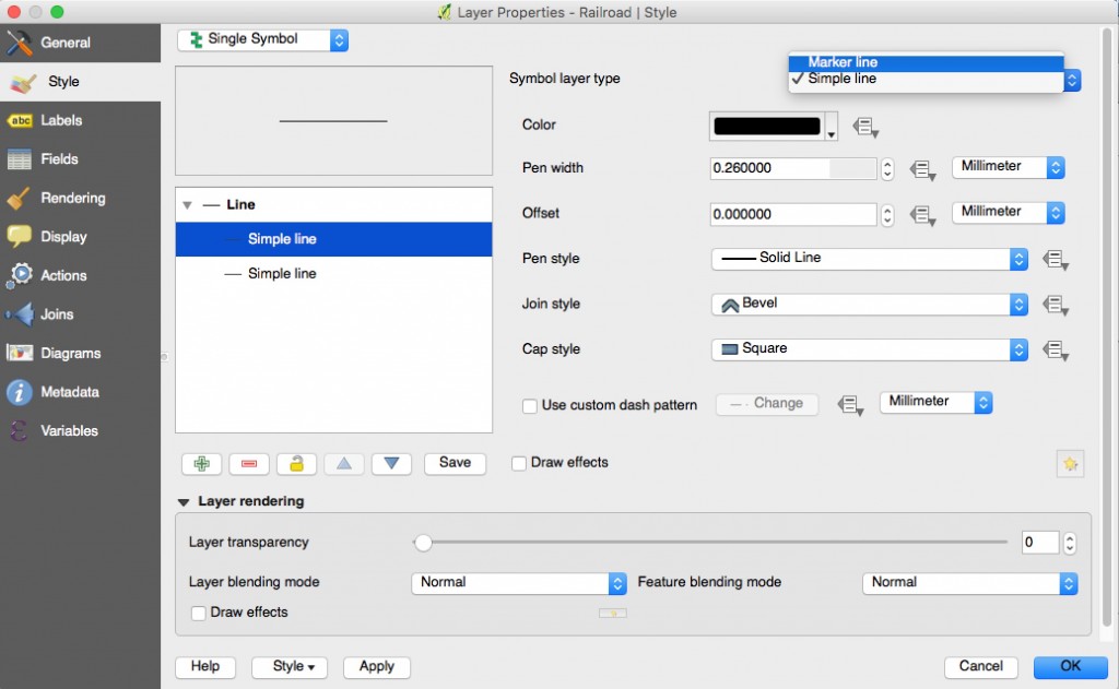
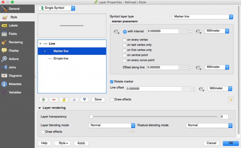
For Railroad, click on the little arrow beside the color box, and you will see an option for “Standard Colors.” Choose black for these lines. Now, click on the little green “+” on the left side of the window, under the area where you see “Line” and below that “Simple Line.” You will see a second “Simple Line” appear. In the upper right corner, in the drop down box for Symbol Layer type, choose “Marker Line.”
Click on the third inset of this new line, “Simple marker,” and choose the vertical line in the box of symbols at right. Change the colors to black, and change the size to 1.
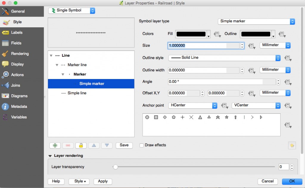
Choose the first in this group, “Marker line,” and change “with interval” to 2.0000. Click OK.
2.5 | Adding Raster Data
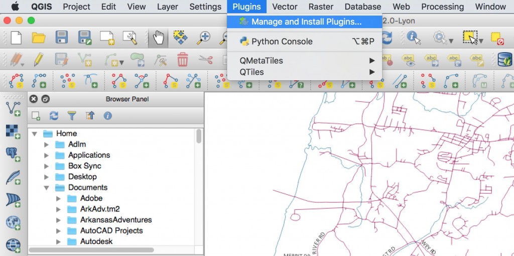
We can easily add tiled raster data, such as Google or Apple Maps or Open Street Maps, by installing a plugin that directly accesses it. We will first need to install the plugin in QGIS. Click on Plugins > Manage and Install Plugins…

In the Search field, type openlayers to search for the OpenLayers Plugin.

Choose that plugin and click Install Plugin.

Click Close to return to the editing screen for the project. In the menu bar, choose Web > Google Maps > Google Streets (or whichever you want to use as a reference).


Return to top ↵
3.0 | Georeferencing an Historic Map
Now we have the context and are ready to georeference an historic map! The image we will be using is a map of Red Hook in 1876 from the New York Public Library. Using QGIS instead of the NYPL MapWarper will allow you to georeference your map without it being on the MapWarper site with the potential for others to move your points or put the map image in the public domain. In short, this will give you more control over your map image.

3.1 | Adding labels to vector layers for reference
Before we start georeferencing, let’s add some labels to the roads for reference. First, we need to check the attribute table to see what the column name is for the road names.
Open the attribute table for the roads layer, tgr36027lkA, by right clicking on the layer in the Layers Panel or by clicking on the attribute table icon in the menu bar.
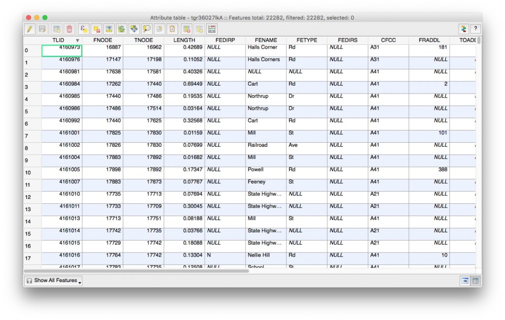
You will see that the name of the street is separate from the kind of road it is. For instance, Halls Corner and Rd are separate columns, fename and fetype. We will want to combine them for the label. Close this attribute table.
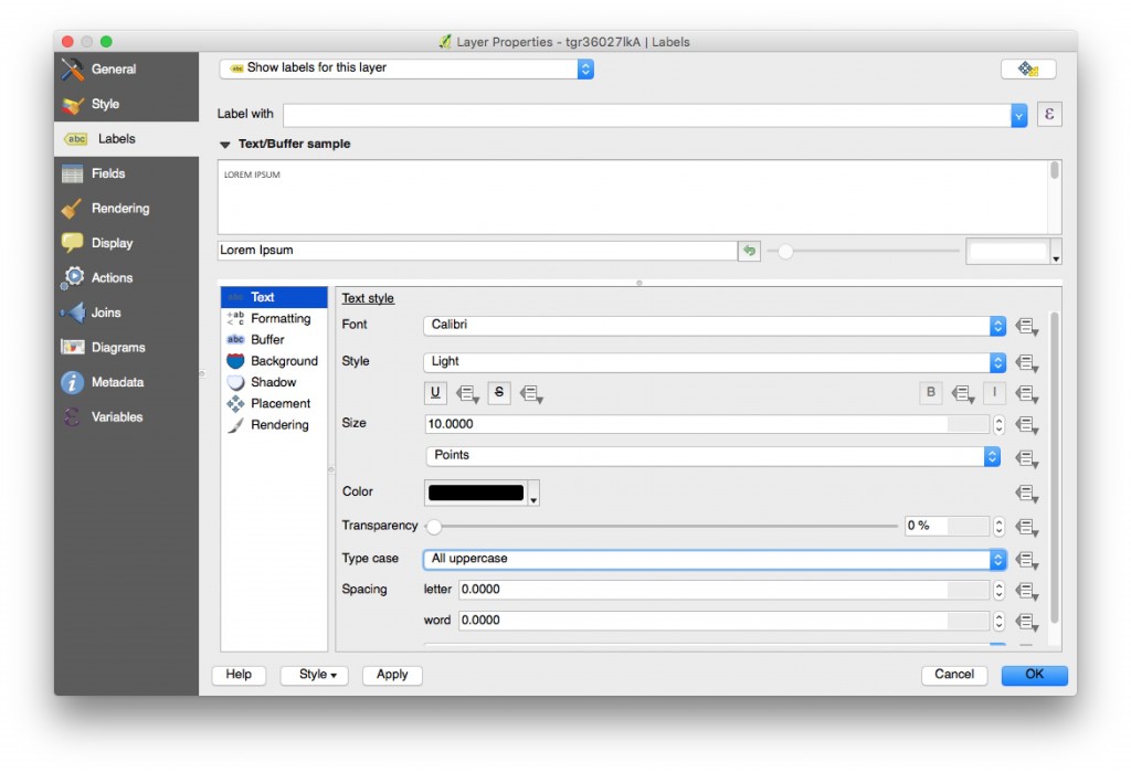
With the roads layer highlighted in the Layers Panel, double click to open the properties panel and choose the labels options. Change your settings to match those below.
For the Label with section, click on the ε to the right to open a “wizard” for building formulas. Under String in the value box in the middle, choose concat to concatenate two strings of text together. You will see it appear in the window to the left and an open parenthesis. Type fename, followed by a comma, followed by an open single quotation mark, hit the space bar to leave a space between the two columns of information, close single quotation mark, followed by a comma, type fetype, close parenthesis. Click OK.
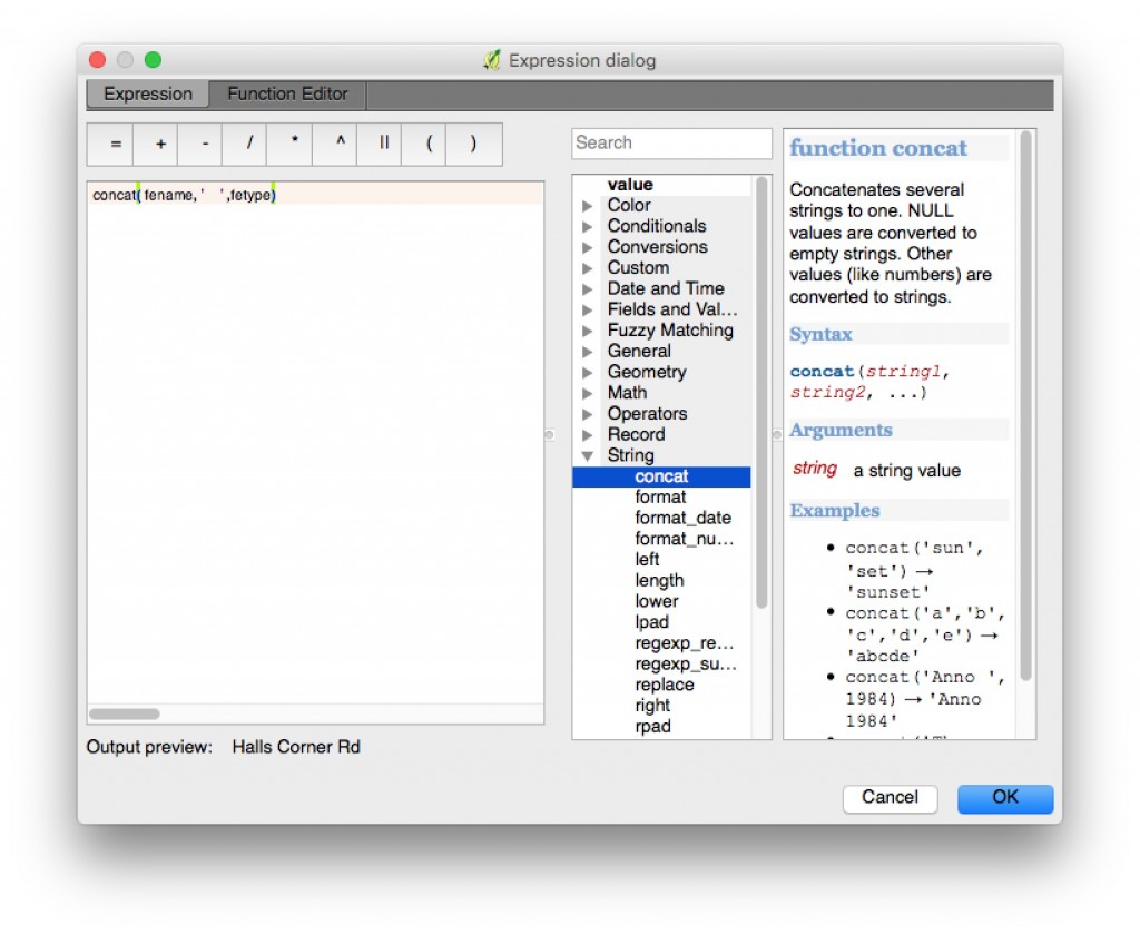
This formula will now appear in the Label with box. You do not have to go through the wizard to build the formula. We did it this way to show you that this tool exists in QGIS if you don’t already know the function you need and its syntax.
Back in the Layer Properties panel, choose the Placement option. Change the placement to Curved so that the labels will bend with the shape of the roads. Click OK.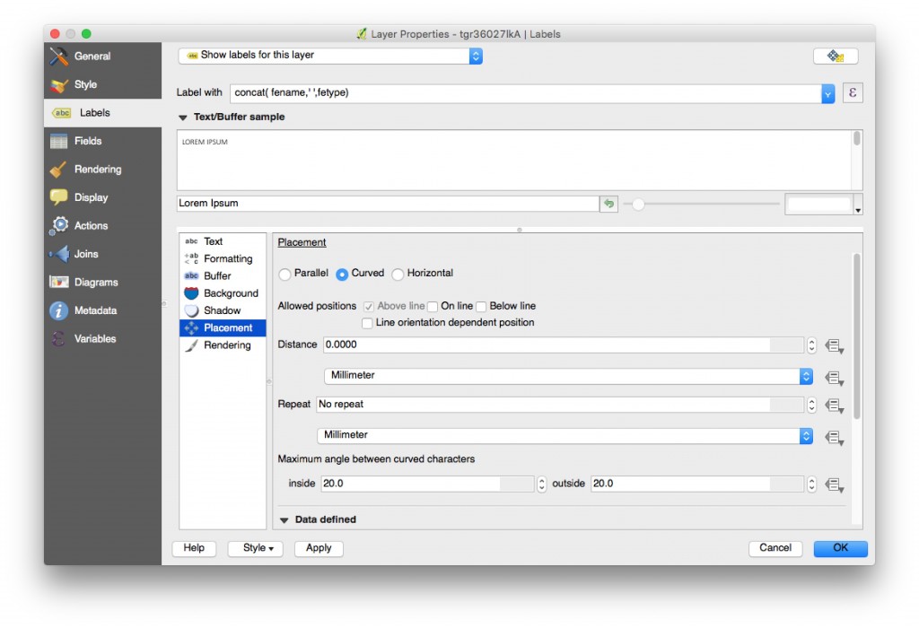
3.2 | Installing Georeferencer plugin
Before we can begin to georeference the historic maps, we will need to install a plugin in QGIS. In the menu bar, choose Plugins > Manage and Install Plugins
When the next window appears, search in the bar at top for georeferencer. You should see the plugin, Georeferencer GDAL. Highlight this plugin, and choose to Install. [note that in the screenshot below the plugin is already installed, thus it will appear differently from yours until you install it] Once installed, close the Plugins window.
3.3 | Georeferencing the Historic Map
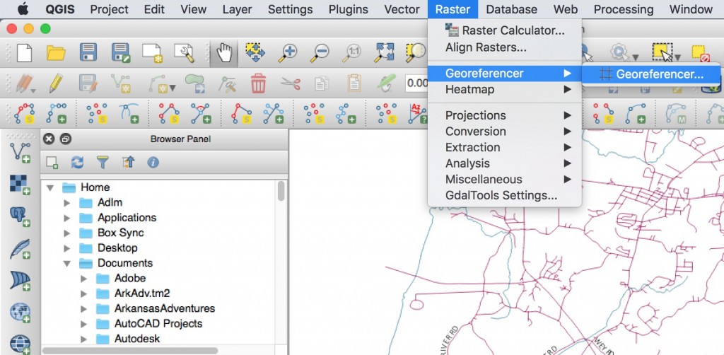
Next, open the Georeferencer GDAL too by choosing Raster > Georeferencer > Georeferencer… This will open a new window.
If this plugin does not appear in your Raster menu, you will need to open the Plugins window again and double check that the box is selected for the Georefrencer GDAL. Note that the check mark will appear light and hard to see. Look closely and be sure that the box is checked.
In the new window, choose the checkerboard icon with the plus sign (Open Raster). Navigate to the saved .jpg of the Red Hook map.

Choose the file, and then be sure to set the projection to match the projection of the project. You can find that in the lower left of the larger project pane where it reads: Render.

In the georeferencer dialogue box for the projection, search for the matching projection and choose it.

Now the work begins in georeferencing. This is a task that requires you to be somewhat familiar with the landmarks on the map. We will use the georeferencer tool to identify points on the vector files we loaded and matching them to points we can identify on the historic map. You will need to zoom in and zoom out and pan around to find these points.
Click on the Add Point icon ![]()
Find a point that is easily recognizable, such as an intersection of roads. Click on it and in the next dialogue box that appears, choose From map canvas to pick the same point on the vector/raster data you have added to the project.

For the best success in georeferencing, try to identify points along the boundaries and some spread throughout the middle.
When you have located several points (as many as you can possibly locate is ideal), you are ready to transform the raster of the historic map. Click on the yellow gear in the georeferencer menu.
![]()
A new window will appear. Match your settings as seen below [for more about these settings see this tutorial].
You will need to choose a filename for your output.
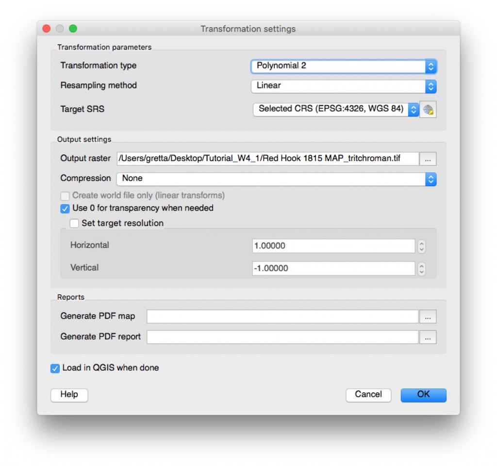
Click OK. You will see a new version of your historic map showing the transformation of the image by lines extending from the points you defined. Click the green arrow to start georeferencing your historic map to your project.
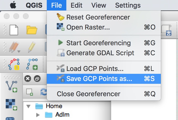
You will need to save your GCP points now, too. To do this, choose File > Save GCP Points as… Save the points in the Tutorial_W4_1 folder, too. Then, close the Georeferencer.
3.4 | Using your geotiff
Now that you’ve saved your geotiff, you can use the first steps in this tutorial to put your map on a basemap and put it online!